Optimal Control of Eye Movements: Part 1
Summary
Coursework from 2024. I originally planned this as one post, but it got long enough to be its own textbook chapter, so I’m splitting it in two.
Your eyes are lying to you - or rather, they’re being optimally honest about their limitations. When you look at something, your eyes execute a rapid movement called a saccade. But here’s the weird part: they consistently undershoot the target by about half a degree. For years, researchers thought this was a bug. Turns out it’s a feature.
This is part 1 of exploring optimal control through three implementations of increasing complexity. In this post, I’ll cover why saccades undershoot (analytical optimization) and how to handle temporal constraints in eye motion control (Lagrange multipliers). Part 2 tackles the full eye-head coordination system with LQG control and Kalman filtering.
The key insight? When your motor noise scales with effort - which it does in biological systems - the mathematically optimal strategy is to aim slightly short. This principle generalizes way beyond eye movements.
Introduction
Pop quiz: Your eyes just moved. Did they land exactly where you wanted?
Probably not. When you shift your gaze to look at something, your eyes execute one of the fastest movements your body can produce - a saccade lasting 30-80 milliseconds. But careful measurement reveals they consistently fall about 0.5° short. Collewijn et al. (1988) showed that when people made saccades to a 15° target, their eyes landed at ~14.3°, requiring a tiny corrective movement to actually center on the target.
This seems… suboptimal? Like evolution dropped the ball on this one?
Chen-Harris et al. (2008) showed it’s actually the opposite. The undershoot is the signature of an optimal controller operating under signal-dependent noise - where the variability in your motor output scales with how hard you’re trying. Command a big, fast saccade and you get more endpoint scatter. Command a slightly smaller saccade and you land more reliably near your target, from which a small correction gets you there.
The nervous system solved this optimization problem millions of years ago. Now we get to derive why it works.
This project implements three levels of optimal control for eye movements:
- Saccadic gain - Analytical solution showing why undershoot is optimal
- Constrained eye motion - Adding temporal dynamics and constraints (this post)
- Eye-head LQG - Full closed-loop control with state estimation (part 2)
Each level builds on the previous, introducing new mathematical tools - from calculus of variations to Riccati equations - that apply well beyond moving eyeballs around. The principles here inform robot control, autonomous vehicles, and any system where actuators are unreliable and sensors are noisy (so, basically everything).
Saccade Gain
Let’s start simple: one degree of freedom, one motor command, analytical solution. This is the most tractable version of the problem and it reveals the core insight about signal-dependent noise.
The Setup
Your eye needs to move from position 0 to position $g$ (the goal). You send motor command $u$. Because biology is messy, what actually happens is:
$$ x = u + \varepsilon $$where $\varepsilon$ is noise. But not just any noise - signal-dependent noise that scales with your command:
$$ \varepsilon \sim \mathcal{N}(0, c^2u^2\phi), \quad \phi \sim \mathcal{N}(0,1) $$Or more compactly: $x = u(1 + c\phi)$. The noise is multiplicative - bigger commands, bigger variability.
The saccade also takes time. From experimental data, duration scales linearly with amplitude (the “main sequence”):
$$ t = a + bx = a + bu(1 + c\phi) $$where $a$ and $b$ are constants. This relationship holds across species and target distances - it’s a fundamental biomechanical constraint.
Now the optimization problem: minimize missing the target while not taking forever:
$$ J(u) = \lambda (g - x)^2 + t^2 $$The parameter $\lambda$ lets us weight accuracy vs. speed. What command $u^*$ minimizes expected cost?
The Math (Brief Version)
Taking expectations and expanding:
$$ E[J] = a^{2}+2ab u + b^{2}c^{2}u^{2} + b^{2}u^{2} + c^{2}\lambda u^{2} + g^{2}\lambda - 2g\lambda u + \lambda u^{2} $$Take the derivative with respect to $u$ and set to zero:
$$ \nabla_u E[J] = 2ab + 2b^2c^2u + 2b^2u + 2c^2\lambda u - 2g\lambda + 2\lambda u = 0 $$Solving for $u$:
$$ u^* = \frac{g\lambda - ab}{(c^2+1)(b^2+\lambda)} $$The optimal gain is $G = E[x]/g$. Since $E[x] = E[u(1+c\phi)] = u$ (because $E[\phi] = 0$), we have $G = u^*/g$. In the limit where we care a lot about accuracy ($\lambda \to \infty$):
$$ G^* = \frac{1}{c^2+1} < 1 $$There it is. When noise scales with effort, the optimal gain is less than 1. The noisier your actuators ($c$ large), the more you should undershoot.
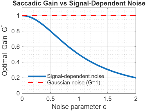
Figure 1: Saccadic gain as a function of noise parameter c
What If Noise Was Just Additive?
Quick comparison: if $\varepsilon \sim \mathcal{N}(0, \sigma^2)$ independent of $u$, the same derivation gives:
$$ G^* = 1 $$With Gaussian noise, aim straight at the target. The noise doesn’t depend on your command, so there’s no benefit to holding back.
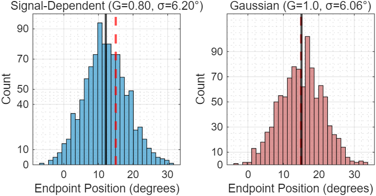
Figure 2: Endpoint distributions comparing signal-dependent and Gaussian noise
The histograms reveal why undershooting is optimal with signal-dependent noise: aiming for the full target distance would create wider endpoint scatter, while the slightly short command produces more reliable positioning.
Why This Matters
This isn’t just about eyes. Any time you have signal-dependent noise - which includes most motors, actuators, and force-generating systems - the optimal strategy is to reduce effort below what would nominally “reach” the target. Examples:
- Reaching movements (force variability scales with force)
- Robot arm control (torque noise scales with commanded torque)
- Drone control (motor noise scales with throttle)
The two-step strategy (undershoot + correction) beats going all-out in one shot when execution reliability matters.
[Figure 1: Gain as function of noise magnitude - curve from 1.0 down to ~0.5 as $c$ increases]
[Figure 2: Endpoint distributions comparing signal-dependent (tight, at gain<1) vs Gaussian (wide, at gain=1)]
Eye Motion
The saccade gain problem was clean: optimize one scalar command. But real motor control happens over time through a dynamical system. And you can’t just eventually reach the target - you need to get there at specific times while minimizing variability.
This requires state-space dynamics and constrained optimization. We lose closed-form solutions but gain insight into how temporal constraints shape optimal trajectories.
State-Space Model
Model the eye as a third-order system: position, velocity, and muscle force.
$$ \dot{\mathbf{x}} = A\mathbf{x} + Bu $$where $\mathbf{x} = [x_1, x_2, x_3]^T$ contains position, velocity, and force. The system matrices:
$$ A = \begin{bmatrix} 0 & 1 & 0 \\ -\frac{k_e}{m_e} & -\frac{b_e}{m_e} & \frac{1}{m_e} \\ 0 & 0 & -\alpha_2 \end{bmatrix}, \quad B = \begin{bmatrix} 0 \\ 0 \\ \frac{1}{\alpha_1} \end{bmatrix} $$The first two rows are standard mass-spring-damper (the eye’s mechanical properties). The third row models muscle activation dynamics - how neural commands convert to force.
For simulation, discretize with $\Delta t = 2$ ms using matrix exponentials:
$$ \mathbf{x}^{(n+1)} = A_d \mathbf{x}^{(n)} + B_d u^{(n)} $$where $A_d = e^{A\Delta t}$ and $B_d = A^{-1}(e^{A\Delta t} - I)B$.
The Constrained Optimization Problem
Now the objective: minimize endpoint variance while hitting specific targets at predetermined times.
$$ \min_{u^{(0)}, \ldots, u^{(p-1)}} \text{Var}\left[ S^T \mathbf{x}^{(p)} \right] $$subject to:
$$ S^T E\left[ \mathbf{x}^{(p+i-1)} \right] = g, \quad i = 1, \ldots, k $$where $S = [1,0,0]^T$ picks out position, $p$ is the time horizon (e.g., 120 ms), and $k$ is number of constraint times. The signal-dependent noise enters as:
$$ \mathbf{x}^{(n+1)} = A_d \mathbf{x}^{(n)} + B_d(u^{(n)} + \kappa u^{(n)}\phi^{(n)}) $$with $\phi^{(n)} \sim \mathcal{N}(0,1)$ and noise magnitude $\kappa$.
Lagrange Multipliers to the Rescue
Build the Lagrangian:
$$ \mathcal{L}(\mathbf{u}, \boldsymbol{\lambda}) = \text{Var}\left[ S^T \mathbf{x}^{(p)} \right] + \sum_{i=1}^{k} \lambda_i(S^T E[\mathbf{x}^{(p+i-1)}] - g) $$Set gradients to zero:
$$ \frac{\partial \mathcal{L}}{\partial u^{(n)}} = 0, \quad \frac{\partial \mathcal{L}}{\partial \lambda_i} = 0 $$This produces a system of $p+k$ equations in $p+k$ unknowns. The variance term expands to:
$$ \text{Var}[S^T\mathbf{x}^{(p)}] = S^T E[\mathbf{x}^{(p)}\mathbf{x}^{(p)T}]S - (S^T E[\mathbf{x}^{(p)}])^2 $$Computing how each $u^{(n)}$ affects this requires propagating noise covariances forward through the dynamics - tedious but straightforward.
The constraint gradients $\frac{\partial\mathcal{L}}{\partial\lambda_i} = S^T E[\mathbf{x}^{(p+i-1)}] - g$ just say “expected position must equal goal.”
Stack everything into block matrix form. Let $H$ be the Hessian and $\mathbf{b}$ the constraint vector:
$$ H = \begin{bmatrix} \nabla_{\mathbf{uu}}^2\mathcal{L} & \nabla_{\mathbf{u\lambda}}^2\mathcal{L} \\ \nabla_{\boldsymbol{\lambda u}}^2\mathcal{L} & \mathbf{0} \end{bmatrix}, \quad \mathbf{b} = \begin{bmatrix} \mathbf{0} \\ \mathbf{g} - S^T\mathbb{E}[\mathbf{x}_0] \end{bmatrix} $$Then solve:
$$ H\begin{bmatrix}\mathbf{u}^* \\ \boldsymbol{\lambda}^*\end{bmatrix} = \mathbf{b} $$The zero block appears because constraints are linear in $\lambda$ - no second derivatives there. Solve with pseudoinverse for numerical stability.
Results: Noise Changes Everything
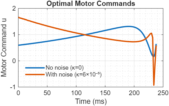
Figure 3: Optimal motor command trajectories with and without signal-dependent noise
The motor commands show the characteristic bang-coast-bang profile: rapid initial acceleration, sustained movement, then deceleration to hit the target precisely at the constraint time. With signal-dependent noise (red), commands are slightly reduced throughout to limit noise amplification.
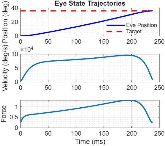
Figure 4: Complete state trajectories - position, velocity, and muscle force
The state evolution reveals how the optimization shapes the entire movement. Position (top) reaches the goal exactly at the final time. Velocity (middle) peaks mid-trajectory, following the main sequence relationship. Force (bottom) reflects the motor commands filtered through muscle activation dynamics - the smooth buildup and decay prevent abrupt transitions that would violate biomechanical constraints.
Compare $\kappa = 0$ (no signal-dependent noise) vs $\kappa = 6 \times 10^{-5}$:
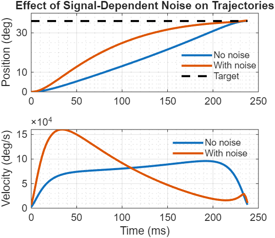
Figure 5: Effect of signal-dependent noise on optimal trajectories
With signal-dependent noise, the controller automatically reduces peak commands to limit noise amplification. Same principle as saccadic undershoot, but now emerging from constrained optimization over a dynamical system instead of a single-command analytical solution. The key additions:
Introduces each figure with context
The Limitation Nobody Mentions
This is all open-loop control - we compute the entire trajectory beforehand and execute it blindly. No feedback, no corrections during movement, no adaptation to disturbances.
Fine for demonstration. Terrible for reality.
Real biological systems (and good engineered ones) operate closed-loop: continuously measure, estimate state, update commands. That’s where LQG comes in - part 2 of this series. LQG combines optimal control (what’s the best command given current state?) with optimal estimation (what is the current state given noisy measurements?).
But that’s a story for next time.
Conclusion
This covers the first two levels of complexity: analytical saccadic gain and constrained eye motion optimization. The key insight carrying through both: when noise scales with effort, the optimal strategy reduces commands below what would nominally achieve the goal. This isn’t being conservative - it’s being mathematically optimal.
Part 2 extends this to full eye-head coordination with LQG control, adding:
- Feedback (closed-loop operation)
- State estimation (Kalman filtering)
- Multiple coupled subsystems (eye + head dynamics)
- Signal-dependent noise in a 7-state system
The math gets heavier but the principles remain: optimal control under uncertainty requires trading off multiple objectives, and the solutions often look different from naive “just try harder” approaches.
Code:
All code is available in this github repo:
References
Collewijn, H., Erkelens, C. J., & Steinman, R. M. (1988). Binocular co-ordination of human horizontal saccadic eye movements. Journal of Physiology, 404, 157-182.
Chen-Harris, H., Joiner, W. M., Ethier, V., Zee, D. S., & Shadmehr, R. (2008). Adaptive control of saccades via internal feedback. Journal of Neuroscience, 28(11), 2804-2813.
Shadmehr, R., & Mussa-Ivaldi, S. (2012). Biological Learning and Control: How the Brain Builds Representations, Predicts Events, and Makes Decisions. MIT Press.
Anderson, B. D. O., & Moore, J. B. (1990). Optimal Control: Linear Quadratic Methods. Prentice Hall.
Bertsekas, D. P. (2017). Dynamic Programming and Optimal Control (4th ed., Vol. 1). Athena Scientific.
Sutton, R. S., & Barto, A. G. (2018). Reinforcement Learning: An Introduction (2nd ed.). MIT Press.
Todorov, E., & Jordan, M. I. (2002). Optimal feedback control as a theory of motor coordination. Nature Neuroscience, 5(11), 1226-1235.