Optimal Control of Eye Movements: Part 2
Summary
Part 2 of coursework from 2024. If you haven’t read part 1, start there - it sets up the problem and motivation.
Open-loop control is dead. Long live closed-loop control.
In part 1, I showed why saccades undershoot (signal-dependent noise makes it optimal) and how to handle temporal constraints (Lagrange multipliers). But everything was open-loop - compute the trajectory beforehand and pray nothing goes wrong.
Reality doesn’t work that way. Your head moves unexpectedly. Someone bumps you. Your state estimates drift. You need feedback - continuous measurement, estimation, and command updates based on what’s actually happening.
This is where Linear Quadratic Gaussian (LQG) control enters. It solves two problems simultaneously: optimal control (what’s the best command given current state?) and optimal estimation (what is the current state given noisy measurements?). The beauty is the separation principle - design each independently, connect them, and the result is optimal.
I implement full LQG for coordinated eye-head movements: 7 states, 2 control inputs, partial observability, signal-dependent noise. Five test cases show how the controller adapts to different noise levels and head restraints without any manual tuning.
Eye-Head Coordination
When One Degree of Freedom Isn’t Enough
Part 1’s eye-only model was educational but incomplete. Real gaze control coordinates eyes and head together. Why?
- Range: Eyes alone can move ~50°, but adding head rotation gives you 180°+
- Efficiency: Large movements split between eyes and head reduce eye muscle fatigue
- Speed: Eyes move first (they’re faster), head catches up
But coordination is hard. You have two coupled subsystems with different dynamics, partial measurements, and signal-dependent noise on both control channels. Open-loop planning is hopeless - you need real-time feedback.
System Architecture
The state vector grows from 3 to 7 dimensions:
$$ \mathbf{x} = [x_e, \dot{x}_e, F_e, x_h, \dot{x}_h, F_h, g]^T $$Eye position/velocity/force, head position/velocity/force, plus the goal. The measurement of interest is gaze = eye + head position relative to target, which is what actually determines where you’re looking.
Each subsystem has third-order dynamics like part 1, but with different parameters:
$$ \begin{gathered} A_e = \begin{bmatrix} 0 & 1 & 0 \\ -\frac{k_e}{m_e} & -\frac{b_e}{m_e} & \frac{1}{m_e} \\ 0 & 0 & -\frac{\alpha_{2e}}{\alpha_{1e}} \end{bmatrix} \\ A_h = \begin{bmatrix} 0 & 1 & 0 \\ -\frac{k_h}{m_h} & -\frac{b_h}{m_h} & \frac{1}{m_h} \\ 0 & 0 & -\frac{\alpha_{2h}}{\alpha_{1h}} \end{bmatrix} \end{gathered} $$The head has larger inertia ($m_h > m_e$) and slower activation ($\alpha_{1h} > \alpha_{1e}$) - moving your head takes more time and energy than moving your eyes. This asymmetry drives the coordination strategy.
Full system dynamics are block-diagonal:
$$ A = \text{blkdiag}(A_e, A_h, 0), \quad B = \text{blkdiag}(B_e, B_h, 0) $$Two control inputs ($u_e$ for eyes, $u_h$ for head), seven states to estimate.
The Observability Problem
Here’s the catch: you can’t directly measure everything. The observation equation is:
$$ \mathbf{y} = H\mathbf{x} + \boldsymbol{\nu} $$where $H = \begin{bmatrix} -1 & 0 & 0 & -1 & 0 & 0 & 1 \\ 1 & 0 & 0 & 0 & 0 & 0 & 0 \end{bmatrix}$ and $\boldsymbol{\nu} \sim \mathcal{N}(0, Q_y)$.
You measure gaze error (first row) and eye position (second row). That’s it. No direct velocity measurements, no force measurements. You have to infer the full state from these partial observations.
This is partial observability, and it’s everywhere in real systems: tracking a rocket from radar returns, localizing a robot from odometry, trading on incomplete market data. You need state estimation, and Kalman filtering is the optimal solution (for linear systems with Gaussian noise).
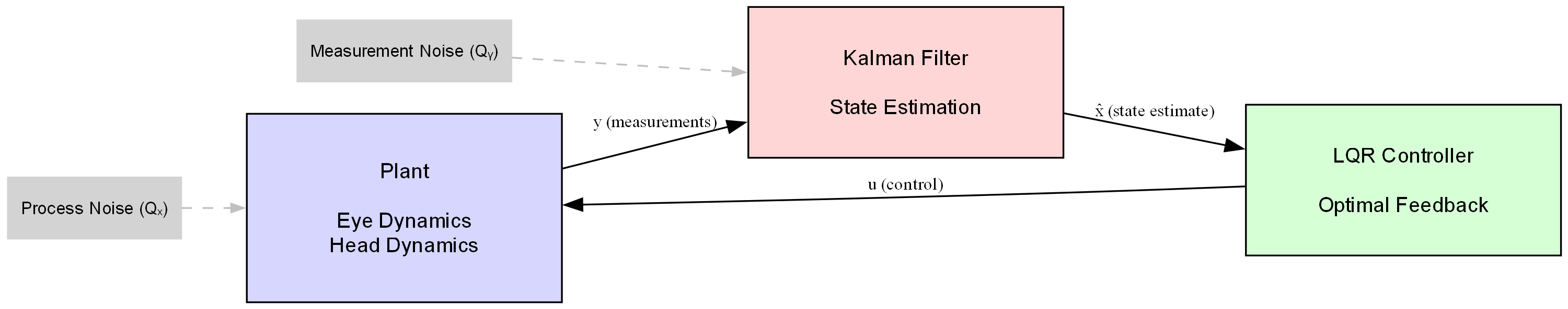
Figure 1: LQG architecture - separation principle in action
The block diagram shows how the three components interact. Process noise enters the plant dynamics, measurement noise corrupts observations, but the Kalman filter and LQR controller work together to maintain optimal performance despite these disturbances.
LQG
LQG solves two intertwined problems:
- Control: Given state $\mathbf{x}$, what command $\mathbf{u}$ minimizes cost?
- Estimation: Given measurements $\mathbf{y}$, what’s the best estimate $\hat{\mathbf{x}}$ of state?
The separation principle says: solve each problem independently, then plug the state estimate into the control law. The resulting controller is optimal for the combined problem.
This is non-obvious and extremely useful. It means you can design your estimator (Kalman filter) without worrying about the controller, design your controller (LQR) without worrying about the estimator, and the combination Just Works™.
The Cost Function
We want to reach a 40° gaze target in ~100ms while minimizing control effort. The cost:
$$ J = E\left[\sum_{t=0}^{p-1} \left(\mathbf{x}^T(t)Q_x\mathbf{x}(t) + \mathbf{u}^T(t)R\mathbf{u}(t)\right) + \mathbf{x}^T(p)Q_f\mathbf{x}(p)\right] $$The terminal cost $Q_f$ heavily penalizes gaze error at the end:
$$ Q_f = H^T T H, \quad T = \begin{bmatrix} 10^5 & 0 \\ 0 & 300 \end{bmatrix} $$This says: gaze error at 100ms is really bad (weight of $10^5$), eye position deviation is less critical (weight 300). Makes sense - the goal is seeing the target, not perfectly centering your eye in its socket.
Optimal Control
Computing optimal feedback gains uses dynamic programming - start at the end, work backward asking “what should I do with $n$ steps remaining?”
The value function $W_x(t)$ represents future cost-to-go from time $t$. It satisfies the discrete-time Riccati equation:
$$ W_x(t-1) = H^T T H + A^T W_x(t)A - A^T W_x(t)BG(t) $$where $T = 0$ before the target time, then takes the value above. The optimal feedback gain at each time:
$$ G(t) = \left[L + B^T W_x(t)B + B^T W_{xe}(t)C_1 B + B^T W_{xe}(t)C_2 B\right]^{-1} B^T W_x(t)A $$The matrices $C_1 = \text{diag}(c_e, 0)$ and $C_2 = \text{diag}(0, c_h)$ encode signal-dependent noise on eye and head commands separately.
This gain matrix $G(t) \in \mathbb{R}^{2 \times 7}$ maps full state to control inputs. It’s time-varying because optimal strategy changes as you approach the deadline - with less time remaining, you need more aggressive control.
Connection to Reinforcement Learning
If this looks like value iteration from RL, that’s because it is. The Riccati recursion is value iteration for a linear-quadratic system:
- $W_x(t)$ is the value function
- Backward recursion is Bellman backup
- $G(t)$ is the policy
LQR is special-case RL where dynamics are linear and costs are quadratic, so we can solve analytically instead of sampling. When you linearize a nonlinear system around a trajectory, solve LQR locally, and iterate, you get differential dynamic programming - a bridge between classical control and modern RL.
Optimal Estimation
While the controller assumes access to $\mathbf{x}$, we only measure $\mathbf{y} = H\mathbf{x} + \boldsymbol{\nu}$. The Kalman filter maintains optimal state estimate $\hat{\mathbf{x}}$ through predict-update cycles:
Prediction - propagate estimate forward through dynamics:
$$ \begin{aligned} \hat{\mathbf{x}}(t+1|t) =& A\hat{\mathbf{x}}(t|t) + Bu(t)\\ S_e(t+1|t)=&AS_e(t|t)A^T+Q_x\\ &+BC_1G(t)S_x(t|t)G^T(t)C_1^TB^T\\ &+BC_2G(t)S_x(t|t)G^T(t)C_2^TB^T \end{aligned} $$The covariance $S_e$ tracks estimation uncertainty. Process noise $Q_x = 10^{-5} \cdot I_7$ represents unpredictable disturbances. The signal-dependent terms show how control actions introduce additional uncertainty.
Update - correct estimate when measurement arrives:
$$ K(t) = S_e(t|t-1)H^T[HS_e(t|t-1)H^T + Q_y]^{-1} $$$$ \hat{\mathbf{x}}(t|t) = \hat{\mathbf{x}}(t|t-1) + K(t)[y(t) - H\hat{\mathbf{x}}(t|t-1)] $$The Kalman gain $K(t) \in \mathbb{R}^{7 \times 2}$ determines measurement trust vs. prediction trust. When $S_e$ is large (uncertain), $K$ is large (trust measurement). When $Q_y$ is large (noisy sensor), $K$ is small (trust prediction).
The covariance update:
$$ S_e(t|t) = (I - K(t)H)S_e(t|t-1) $$These forward-propagating covariances track how uncertainty evolves, while the backward-propagating value function tracked future costs. Connect them through the separation principle: $u = -G\hat{\mathbf{x}}$, and you have optimal LQG control.
The Circular Dependency Problem
Here’s where it gets tricky. The feedback gains $G(t)$ depend on covariances $S_x(t)$ that evolve forward in time. But those covariances depend on $G(t)$ through the closed-loop dynamics. Similarly, Kalman gains $K(t)$ depend on covariances that evolve under the control policy.
Break this circular dependency through iteration:
- Initialize $G^{(0)}(t) = 0$ (no control)
- Forward pass: compute $K^{(1)}(t)$ given $G^{(0)}$
- Backward pass: compute $G^{(1)}(t)$ given $K^{(1)}$
- Repeat until convergence (~10 iterations)
Both problems are convex, so this converges. Each iteration improves the control policy given current estimator and improves estimator given current controller. After convergence, you have time-varying schedules $G(t)$ and $K(t)$ implementing optimal LQG control.
Stress-Testing the Controller
To see how LQG adapts to different conditions, I ran five scenarios varying noise magnitude and head constraints:
Case 1: Baseline: No signal-dependent noise ($C_1 = C_2 = 0$), no head hold
Establishes performance with only process and measurement noise.
Case 2: Small Signal-Dependent Noise: $C_1 = C_2 = \text{diag}(0.01, 0.01)$, no hold
Realistic noise where variability scales modestly with effort.
Case 3: Large Signal-Dependent Noise: $C_1 = C_2 = \text{diag}(2.0, 2.0)$, no hold
Exaggerated noise to stress-test adaptation.
Case 4: Small Noise + Short Head Hold: Noise as case 2, 50ms head immobilization
Simulates brief external head restraint.
Case 5: Small Noise + Long Head Hold: Noise as case 2, 100ms head immobilization
Extended restraint requiring eye-only compensation.
Each case: 50 trials with different noise realizations. Head hold implemented by forcing $\mathbf{x}(4:5) = 0$ during constraint period.
Results
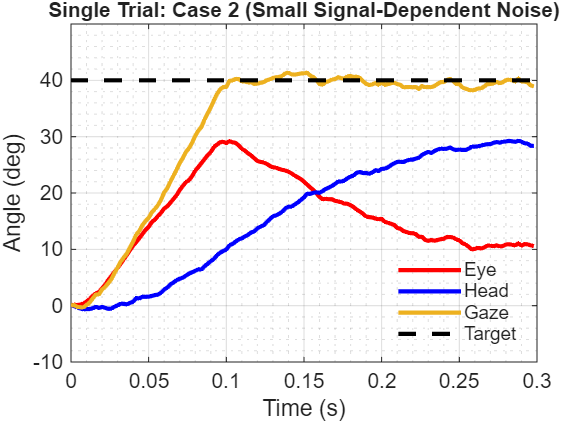
Figure 2: Single trial from Case 2 - coordinated eye-head movement
This single realization shows the characteristic coordination pattern. Eyes move first because they’re faster (lower inertia, quicker activation). The head follows with slower dynamics but eventually carries more of the total displacement, allowing the eyes to return toward center in the orbit. By 300ms, gaze is stable on target with the load distributed between eye and head.
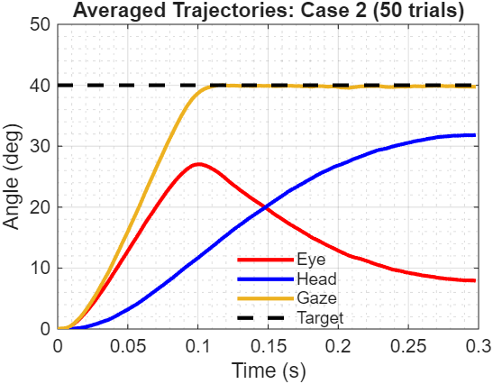
Figure 3: Averaged trajectories reveal the underlying control strategy
Averaging across 50 trials removes stochastic noise, exposing the deterministic component of the optimal policy. The smooth curves show that the controller consistently implements the same basic strategy: rapid eye movement initiation, gradual head contribution, coordinated convergence to target. The gaze trajectory (yellow) shows remarkably low variance - the controller reliably hits the target despite noisy actuation.
The eye-dominates-early-then-head-catches-up pattern is automatic - not programmed, but emerging from the different dynamics and the optimal cost-to-go computation.
Comparing across noise levels:
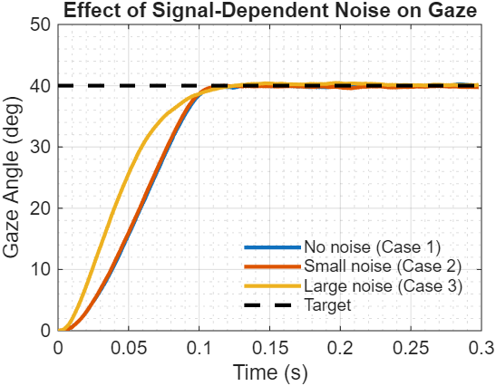
Figure 4: Signal-dependent noise changes the optimal strategy
The controller automatically adapts its aggressiveness to noise magnitude. With no signal-dependent noise (Case 1), it executes rapid movements - there’s no penalty for large commands. Small noise (Case 2) slightly moderates the strategy. Large noise (Case 3) forces significant adaptation: the controller reduces motor commands throughout the trajectory to limit noise amplification, accepting longer movement duration in exchange for reliable endpoint positioning.
Same principle as saccadic undershoot, but now emerging from LQG optimization in a 7-state system instead of analytical derivation for a scalar command.
Head hold cases show compensation:
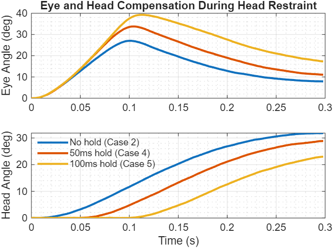
Figure 5: Automatic compensation for head restraints
The head hold cases demonstrate robust adaptation to unexpected constraints. When the head is immobilized (Cases 4-5), the Kalman filter quickly infers that commanded head movements aren’t producing actual motion - the prediction error signals model-plant mismatch. The controller responds by increasing eye commands to maintain gaze on target.
After head release, the system smoothly redistributes the load: the head accelerates to catch up while the eye returns toward a more comfortable position in the orbit. Longer hold periods (Case 5, 100ms) require larger initial eye compensation, but the LQG framework handles both scenarios without retuning or explicit reasoning about constraints. This adaptation emerges purely from optimal state estimation and feedback control.
During restraint, the Kalman filter rapidly infers head states aren’t evolving as predicted (commanded movements produce no motion). The controller, receiving updated estimates, compensates by increasing eye commands. This adaptation - no explicit constraint reasoning required - emerges from optimal handling of model-plant mismatch.
What This Demonstrates
Three key principles of optimal feedback control:
1. Controllers should adapt aggressiveness to actuator reliability
When noise is high, reduce effort. Not conservative - mathematically optimal.
2. Partial observability requires principled state estimation
Kalman filtering optimally fuses predictions with measurements despite sensor noise.
3. Feedback handles unanticipated disturbances automatically
No need to model all possible perturbations - just observe deviations and respond optimally given current estimates.
The progression from part 1’s open-loop to this closed-loop implementation shows how control problems grow: static → dynamic, full observability → partial observability, deterministic → stochastic. Each level requires new math (Lagrange multipliers → Riccati equations → Kalman filtering) but the principles carry through.
Takeaways and Connections
Optimal Control Principles
Signal-dependent noise changes everything. When execution variability scales with effort, “trying harder” backfires. This appears in:
- Biological motor control (muscle force variability)
- Robot torque control (amplifier noise)
- Drone throttle (motor noise)
- Any system where actuator reliability degrades with command magnitude
The saccadic gain analysis proved this analytically. LQG showed it emerging automatically from numerical optimization. Same principle, different levels of complexity.
RL Connection (Deeper This Time)
The mathematical structure of LQG directly parallels RL:
- $W_x(t)$ = value function (expected future cost)
- Riccati recursion = value iteration (Bellman backup)
- $u = -G\mathbf{x}$ = policy (state → action mapping)
Model-based RL (Dyna, PILCO) learns dynamics then applies optimal control. Model-free RL (Q-learning, actor-critic) approximates value functions directly from experience. Both converge to LQG solutions when the system is actually linear-quadratic.
When do you use which?
- LQG: Linear dynamics, quadratic costs, perfect model → closed-form solution
- RL: Nonlinear, arbitrary costs, unknown model → sample and learn
- Hybrid: Linearize around trajectories, apply LQG locally, iterate (iterative LQG, DDP)
Practical Implementation
Building these controllers taught me:
- Matrix exponentials for discretization (numerical stability matters)
- Riccati recursion (backward dynamic programming)
- Covariance propagation (forward through nonlinear noise)
- When pseudoinverses are needed
- Iterative refinement for coupled problems
The iterative coupling between Kalman and feedback gains illustrates a general principle: many optimal control problems decompose into subproblems that must be solved jointly. Recognizing structure that admits decomposition vs. requiring joint solution is learned through examples.
What’s Missing
These implementations assumed perfect model knowledge (the $A$ and $B$ matrices). Real systems must learn dynamics from experience:
- Adaptive control: Estimate parameters online, update gains
- System identification: Fit models from data
- Model-based RL: Learn dynamics through interaction
Real oculomotor plants have nonlinearities - muscle force-length curves, saturation limits, nonlinear vestibulo-ocular reflexes. Extensions:
- Iterative LQG: Repeatedly linearize around trajectories
- Differential dynamic programming: Local quadratic approximations
- Model predictive control: Online optimization at each timestep
Scaling to higher dimensions (reaching, locomotion, multi-agent) introduces computational challenges but the principles remain: model uncertainty, estimate states, compute optimal feedback.
Conclusion
This completes the progression from analytical optimization (saccadic gain) through constrained open-loop control (eye motion) to full closed-loop LQG (eye-head coordination).
The key insight persists: when noise scales with effort, optimal control looks different from naive approaches. You undershoot. You reduce commands. You accept longer duration for tighter distributions. Not being conservative - being optimal.
LQG provides the machinery to implement this automatically: Riccati recursion for optimal feedback, Kalman filtering for optimal estimation, separation principle connecting them. The math gets heavier but enables handling partial observability, stochastic disturbances, and multiple coupled subsystems.
These tools generalize beyond moving eyeballs: robot control, autonomous vehicles, financial trading, any domain where you must act optimally under uncertainty with unreliable actuators and noisy sensors.
Which is basically everything.
Code:
All code is available in this github repo:
References
Collewijn, H., Erkelens, C. J., & Steinman, R. M. (1988). Binocular co-ordination of human horizontal saccadic eye movements. Journal of Physiology, 404, 157-182.
Chen-Harris, H., Joiner, W. M., Ethier, V., Zee, D. S., & Shadmehr, R. (2008). Adaptive control of saccades via internal feedback. Journal of Neuroscience, 28(11), 2804-2813.
Shadmehr, R., & Mussa-Ivaldi, S. (2012). Biological Learning and Control: How the Brain Builds Representations, Predicts Events, and Makes Decisions. MIT Press.
Kalman, R. E. (1960). A new approach to linear filtering and prediction problems. Transactions of the ASME–Journal of Basic Engineering, 82(Series D), 35-45.
Anderson, B. D. O., & Moore, J. B. (1990). Optimal Control: Linear Quadratic Methods. Prentice Hall.
Bertsekas, D. P. (2017). Dynamic Programming and Optimal Control (4th ed., Vol. 1). Athena Scientific.
Sutton, R. S., & Barto, A. G. (2018). Reinforcement Learning: An Introduction (2nd ed.). MIT Press.
Todorov, E., & Jordan, M. I. (2002). Optimal feedback control as a theory of motor coordination. Nature Neuroscience, 5(11), 1226-1235.
Stengel, R. F. (1994). Optimal Control and Estimation. Dover Publications.
Athans, M. (1971). The role and use of the stochastic linear-quadratic-Gaussian problem in control system design. IEEE Transactions on Automatic Control, 16(6), 529-552.