Poisson tiles: part 1
Summary
The motivation for this mini-project was to not only get more familiar with working with $\tt{pygame}$ but also to give myself a playground that I could hook into other packages like $\tt{networkx}$. I also wanted to practice generating fractals. While looking over old notes, I came across the rules for a random process that looked interesting to visualize and potential to become fractal-like.
Introduction
Simeon Denis Poisson lived between 1781-1840 during the tail end of the Age of Enlightenment, a time period characterized by a shift towards the pursuit for knowledge. This was a time of innovation with the creation of the bittersweet invention of the cotton gin and the seminal of the world’s first soft drink. Contributing mostly to physics, it was during his work on La Probabilitie des Jugements that would lead him to the Poisson distribution.
Background
A Poisson distribution is a probability distribution that describes how many occurrences of something you would expect in a fixed interval of time. This number of expected occurrences is often called lambda $\lambda$.
Something with an appearance that can be described with a Poisson distribution is called a poisson process and they arise all over the place like in the arrivals of people to a queues. You can see some cool examples of poisson processes here where you will see that they’re actually quite common!
The probability that, in a fixed time interval, you see $k$ occurrences of something has probability mass function(pmf):
\begin{equation} \Pr(X=k)=\frac{\lambda^ke^{-\lambda}}{k!} \end{equation}
The expected value of this pmf is $E\left(X\right)=\lambda$. In other words, we expect to see lambda number of occurrences on the average.
We can do other things with this distribution. For example, instead of thinking about time we could think about space and play around with these occurrences being either discrete or continuous. Problems like these have important physics applications and can be seen in nuclear decay problems.
In the book Random Networks for Communications by Massimo Franceschetti and Ronald Meester, in the introduction to continuous network models in chapter 2, we’re introduced to the idea of a “somewhat random” point process on a plane with the following specifications:
1. Stationarity - the distribution of the nodes in a region of the plane is the same under any sliding of the region to another part of the plane.
2. Independence - the number of nodes in separate regions won’t affect each other.
3. Absence of accumulation - Only a finite number of nodes in any bounded region can appear.
The book also describes a way to construct such a square in a plane described by:
\begin{equation} p = \frac{\lambda}{n^2} \end{equation}
With probability $p$ and expected value $\lambda$ and number of squares $n$ resulting in $n^2$ sub-squares.
For proof of concept, I’ve simplified this problem down to a framework that can be adapted to such a somewhat random point process in the plane. The model simplification is that most 1 square can appear and the regions are defined with respect to a bounded area of the plane.
So, instead of working with regions, we work with sub-divisions of the plane. This problem is a proper subset of the problem with true stationarity. We’ve fixed our capped Poisson distribution.
Methods
The entire code was written in $\tt{python}$, $\tt{itertools}$ and $\tt{random}$ and visualized using $\tt{pygame}$. Code was written in visual studio code but can be done with any text editor. The repository will be available on github.
Poisson Tile
We define such a subdivision of the plane with properties above and probability of appearing defined above to be a Poisson tile
The individual Poisson tiles were defined by an object with methods for where it is to be instantiated, the probability of it appearing and an update method. The tile sizes were computed using the window size and the $n^2$ number of sub squares desired. The probability that a point appears in the tile is given by equation 1.
Computation and Algorithms
Calculations were performed in two main steps to compute: (1) the centers of instantiation for each square given $n$ and the screen size and (2) the translation required to shift the square to the correct part of the plane. These partitions of the plane are visualized using separate calculation of horizontal and vertical grid lines generated in a separate function.
Calculation of Centers
The centers were determined by finding the midpoint of the sub-squares at the $n$ level excluding the end points, and then taking all 2-ple combinations of these midpoints.
So, let $C_n$ be the set of centers for level $n$ with $n$ elements excluding endpoints of $0$ and $E$ the edge. An algorithm that maps:
\begin{equation} C_n\times C_n\rightarrow(n,n) \end{equation}
and returns a list which contains all centers achieved with $\tt{itertools}$. Due to the symmetry of the square, these tuples define each midpoint of each sub-square.
Calculation of Translation
Due to how $\tt{pygame}$ makes a surface and a rect, I had to translate the rect object in order to slide each sub-square into its correct subdivision of the plane. This subdivision is what is subsequently visualized through the grid lines in the final computation.
Offset called $\delta$ were calculated given the screen size and the $n$ number of squares required. After calculation the squares were translated along the x-axis first and then increment along the y-axis one until all squares were placed. By taking advantage of how the centers were computed I only had to make sure that these translations were assigned in the same order as the centers were computed.
Results
change of lambda constant $n$
In this part of the simulation the number of tiles is held constant while the lambda variable is changed. The simulation shows that as $\lambda$ increases from $1\rightarrow 16\rightarrow 32\rightarrow 64$ the more frequently the points being to appear in the tiles. Alternatively, this can be seen as the probability increasing from $\frac{1}{64}$, to $\frac{1}{4}$, to $\frac{1}{2}$ to $1$. This is makes it clear as to why more squares being to appear because the probability or each tile having a square appear increases. Conversely, the point in the tile appears less frequently while $\lambda$ decreases.
change of $n$ with constant $\lambda$
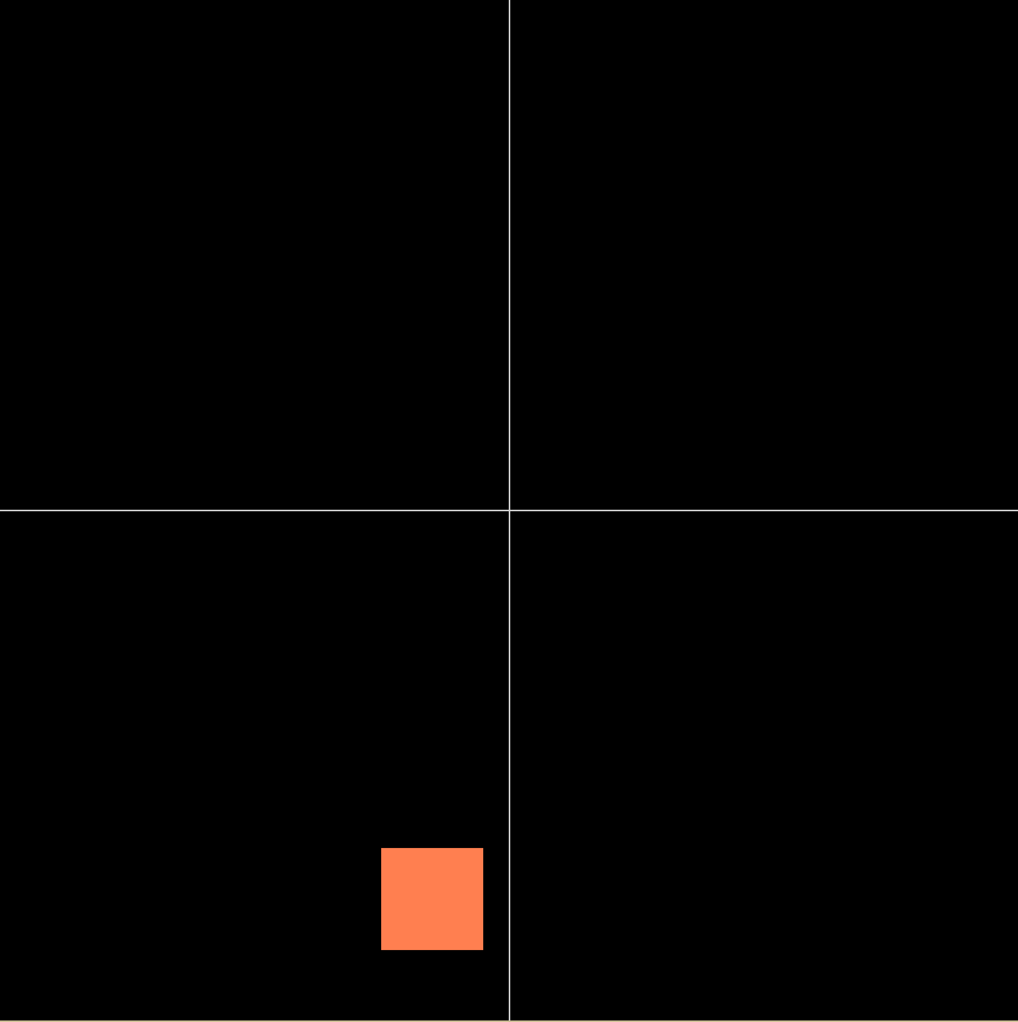
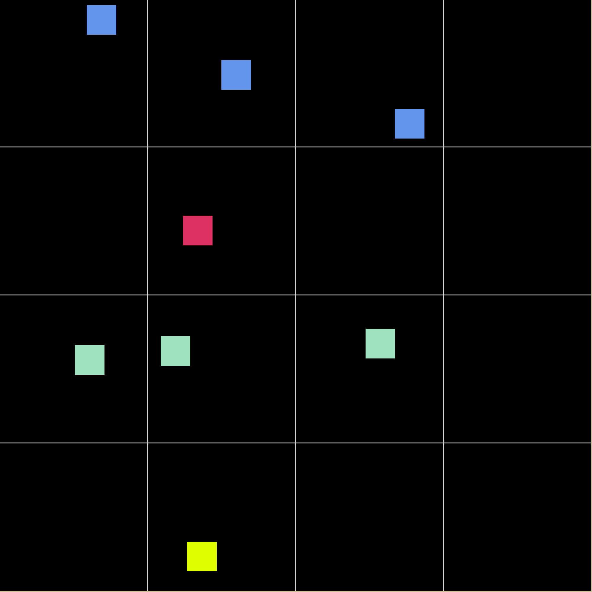
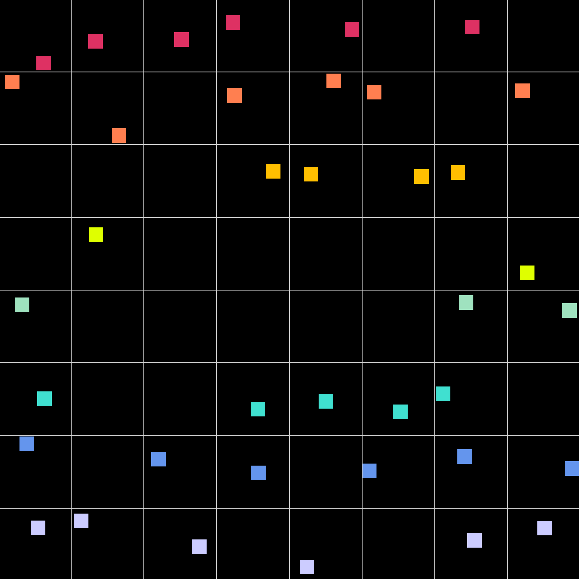
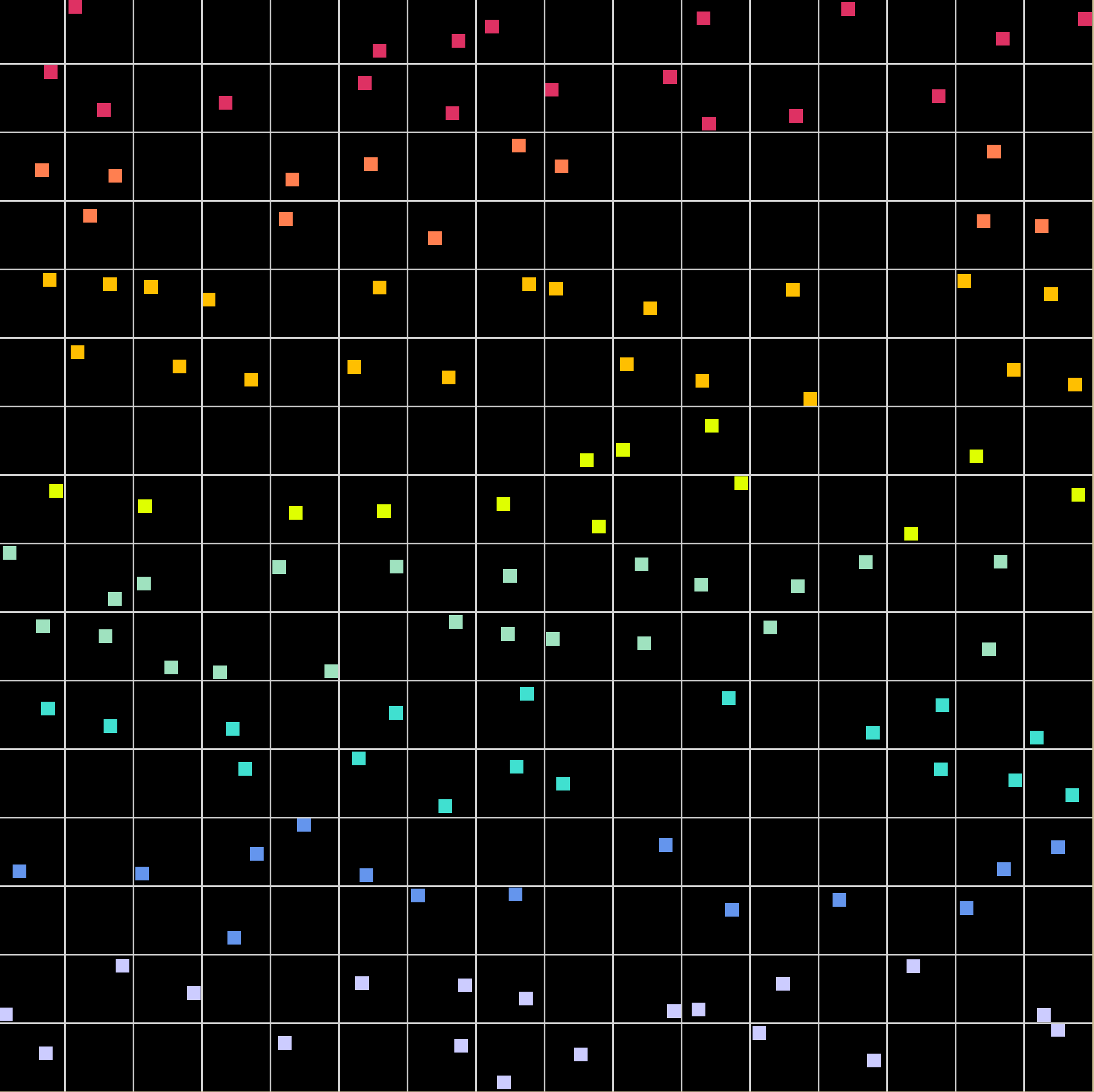
Here is how the simulation handles having various n’s with a fixed tolerance of $\lambda = n^2$ and so the point will always appear in the square. In order from left to right, top to bottom, we have $n=1,2,3,4$. You can see that for $n$ we have $n^2$ tiles appearing. This means that the program can become very computationally expensive to view very quickly. My computer can handle up to at least 50 but at 100 the program fails due to a divide by zero error that comes from floating points being forced to 0 for very large $n^2$.
constant ratio change


Here some patterns produced by the simulation with a constant ratio change of $\lambda = n^2/2$ for $n=1,2,3,4$. With a probability of 50% a dot appears in a tile. Here we can see that we get about half the tiles with a point appearing inside of them while the other half of the tiles do not have a point appearing.
Discussion
It’s pretty cool that for a set $\lambda$, the entire display is generated from a single parameter $n$ $F(n)$ = program. In future updates, I want to rewrite this program to take advantage of it being run with \tt{pygame}. It should be able to be run as an executable that allows you to select an $n$ and view the image. I would also like to have it return basic statistics ater including counts for the number of times a point appeared in a square, the average number of points per cycle etc.
Simplification and improvements
As stated before, these tiles are a simpler version of what I wanted to make since I was a lot busier than I wanted to be. The result is that instead of being Poisson tiles they can actually be seen as Bernoulli tiles. In other words, the simulation can be taken as a binomial distribution of $n^2$ trials and $p$ of appearing. In the future I will remove the simplification and make the poisson tiles I had initially set out to make.
There are some simplifications that can be made in the code in order to make it both run faster and more efficiently. This is would be nice to see exactly how high an $n$ I can run on my computer. This is also a question of how small I can divide the squares by for as $n^2$ increases $\frac{1}{n^2}$ gets closer and closer to zero resulting in a nasty divide by zero error.
Finally, in the future, I would also like to extend this 2D visualizaiton to a 3D visualization as well as fix a sound issue that makes listening to the simulation unbearable for large $n$. This might be a problem of the different channels used in $\tt{pygame}$
Conclusion
This was a fun mini-project. I’ll put it on hold for now because there’s a different one I’d like to start. But I definitely want to come back and make improvements on this. Simulations like these are often done with graphs and can be used in the context of network theory to make comparisons. If the simulation is random-enough we can compare it to another thing and see if it is also random enough and if it isn’t we can ask why. This comes up in things like percolations, links between servers or even the spread of memes on twitter.