Yes/No Hebrew CNN Classification

Summary

Sounds are cool because they’re just a type of signal. Signals are often better understood in their spectrogram form. All of this information can be used by a neural network to learn something. In this case, it learns to identify a word (either a yes or no) by its spectrogram.

All code is available on my github or the colab notebook here

Background and Motivation

I’ve been interested in machine learning and neural networks since my exposure to it during a computational neuroscience class. Although I see it as a type of statistics, it is an incredibly useful and exciting area that has had many promising applications. They’re used in everything from microcontrollers to translators. Right now I’m specifically interested in their use in identifying, producing and understanding language. Each of these tasks seem very similar in people but are quite different for a neural network. Identification and key word recognition tasks are vital for voice activated devices and smart assistance devices.

Additionally, thanks to the ease of access of voice data, I thought it would be a good place to start to explore techniques in processing these data in neural networks. To this end, I took the first dataset I could find on openslr and decided to do some work with it over the thanksgiving weekend.

This was a dataset of yeses and noes in hebrew. I completed this project without hearing what the audio sounded like. Here is an example of an audio file of the speaker saying yes and no in Hebrew. The audio is labeled so that 0 is a no (לא) and 1 is a yes (כן). Or in Hebrew, לא and כן.

Introduction

Convolution neural networks (CNN) are often used in image recognition tasks and are good at finding patterns in images. In computer vision, images are understood as two dimensional arrays of pixel values called channels. In colored images, there are 3 channels while in grayscale or black and white images there is only 1. Since the spectrogram reveals more information about the sound wave than the sound or it Fourier transform alone, they are useful tools in sound processing and provide useful information about the relationship between the frequency of a signal and time. It is this general nature that allows them to unify everything from gravitational waves and music production.

It is also this reason that turns the study of sound into a study of pixels and the motivation for the use of CNNs to process them. There are other ways of identifying sound without going into the frequency domain of the signal like using wavelets. However, the goal of this is to practice using neural networks and so CNNs will be the tool of choice.

Methods

Since the data fed into the model are spectrograms, the independent variables are 2 dimensional matrices with a single value in each coordinate. Since gray-scale images are the same, classification using a convolutional neural network (CNN) is reasonable.

The spectrograms were made using the short-term fast transform with parameters: 256 fast fourier transforms, window length of 256 and 50% overlap slides windowed using the hann window. The resulting matrix was made real valued by taking the modulus of the complex values across each computed array and a final value was computed by taking the natural log of this value. The resulting arrays were used for analysis and computation.

Data points were created by searching minimum energy values and sectioning spectrograms.

As the CNN is not fully connected, we have to make sure that the input size of each image has the same dimension. This was accomplished by padding the axis representing time with a frequency of 0 based on the longest time-segment across all spectrograms.

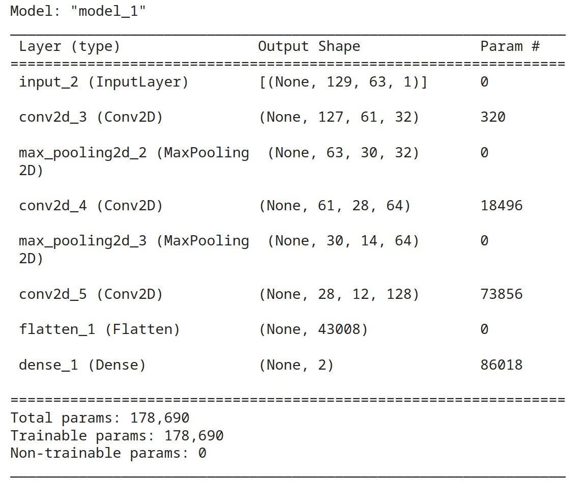
The final layer is a fully connected network of length 2 with a softmax activation.

The optimizer for the classification was root mean squared propagation with sparse categorical cross-entropy loss.

Results

Exploration

Even without knowing what the words mean, visual exploration of the data reveals that there are clear differences in the spectrograms for a yes or a no.

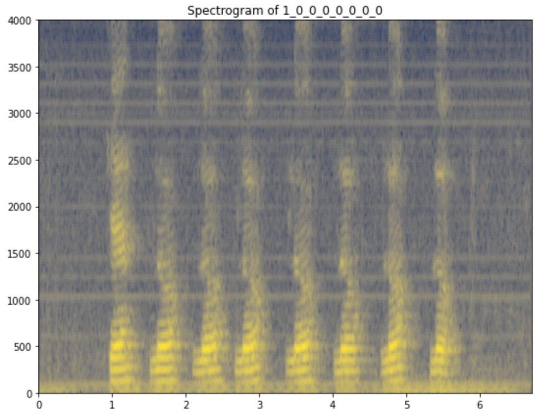
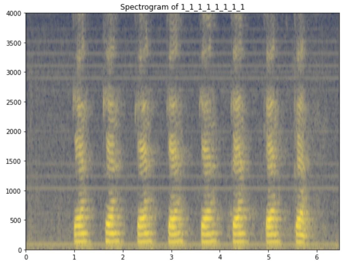
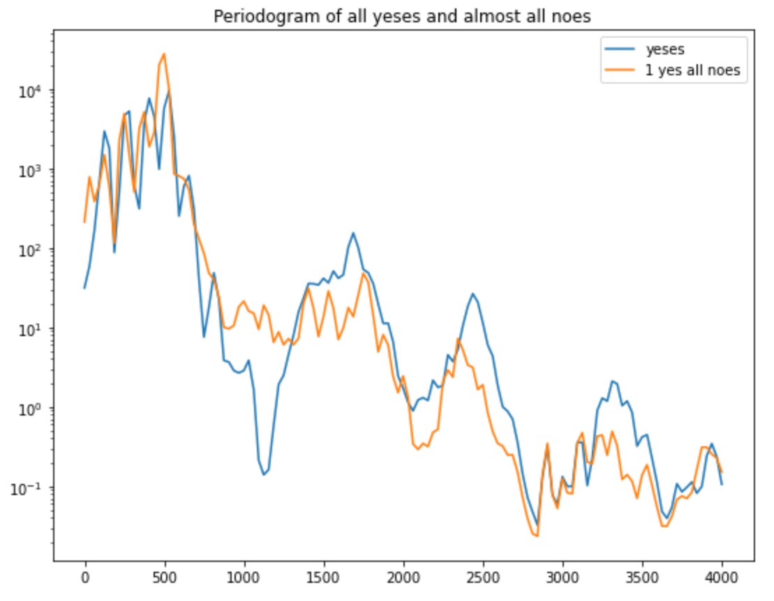
These differences are also found in the periodogram of each signal. The figure below shows that yes has little power contribution from frequencies between 1000Hz and 1250Hz when compared with no signals.

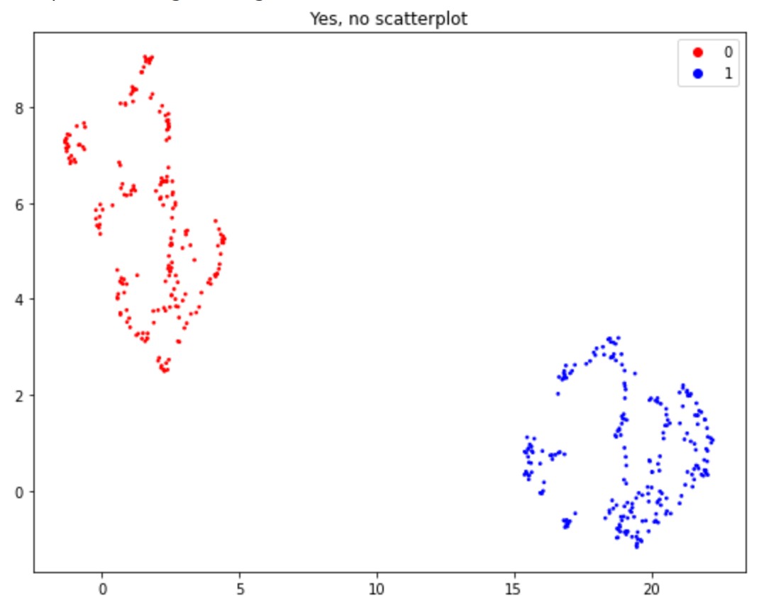
The spectrograms were sectioned into padded windows equal size. These data points were viewed using UMAP, a dimesionality reduction algorithm. It is clear from the figure that there are 2 clusters and the points are well separated between them. However, there is more variation within the no (red points) cluster.

Performance

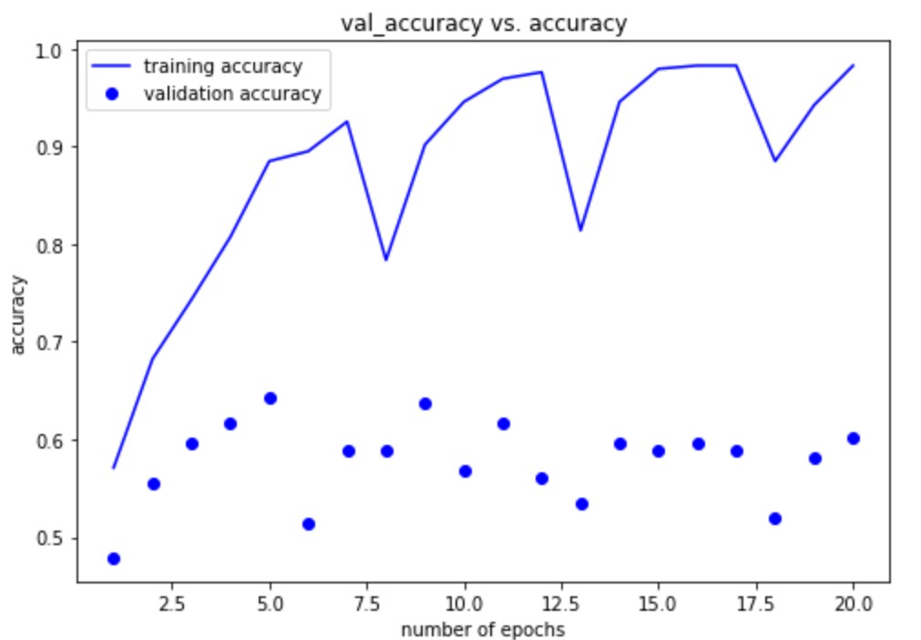
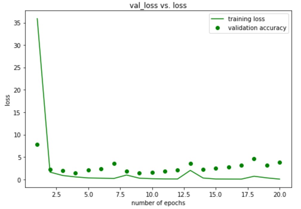
The model was trained with a batch size of 32 and 20 epochs. The model was then tested on the out of sample validation test set. It is clear that the model reaches its best within 5 epochs.

Discussion

The most challenging part of this project, like in any data science project, is the preparation of the data set for the tool being used. Since the goal of this project was to classify the utterance using its spectrogram, the approach I am taking is to feed the neural network batches of labeled spectrograms containing only a yes or a no.

The spectrogram representation of a sound is only as well defined as how little noise is present. This is what makes isolation of the sounds in this form difficult. Often a lot of pre-processing is required to produce a clean representation of sound.

One approach might be to slice at intervals where the sound in decibels is minimal. This is a fair approach and follows how you hear sound. However, when noise is introduced, these points are not well defined as it is possible to have noisy data that competes on a similar decibel level as the signal of interest. An improvement on this approach might be taking averages. This could be across time segments, frequency bins or by passing kernels that compute local means or medians of pixel values.

They still have the drawback of having to reduce the noise in the spectrogram sufficiently enough to process the signal.

Since the goal of this project was just to classify the data set using a neural network, there is no cleaning of the data; however, in practice this is a crucial step to ensure that the signal will be processed by the network.

Future Directions

The main challenges for this project were data cleaning and parsing. However, since the focus of this project was on the data processing aspect, little data cleaning was done and the main obstacle was pairing the labels with the correct spectrogram. As addressed in the challenges section, there are a variety of ways that a spectrogram can be sliced but the naive ways suffer from being imprecise.

Specifically, designating the boundaries for where a signal begins and ends is difficult. In linguistics, this is made more clear by using mel frequency cepstral coefficients (MFCCs) to bin frequency information into ranges that are more comparable with how humans perceive sound. This leads to the obvious first step of providing MFCC scaled data to the network as opposed to log-scale data and comparing how this affects both the network and the parsing.

As mentioned above, another area that needs to be addressed is the lack of data cleaning. Spectrograms being types of image matrices make it a good candidate for kernel filters to reduce noise in the spectrogram. Moreover, determining a decibel threshold for a noise gate could also improve accuracy on out of sample word identification tasks.